In many applications a drift components is added to the Brownian motion.
The easiest example is a random walk where the step to the left is of a different likelihood that to the right. . This results in a mean value which is no longer zero.
The stochastic differential equation adds a deterministic drift term to the diffusion term of the Wiener process. b denotes the drift coefficient.
![]()
![]()
The solution of the above stochastic differential equation is the Wiener process with drift:
y(t) can be seen as a stochastic variable. Realizations of y(t) are representations of the process. The expectation value for y(t) and ln y(t) can be compute as shown below.
![]() The first order expectation value for y(t) is as following:
The first order expectation value for y(t) is as following:
y0 represents the displacement a t0.
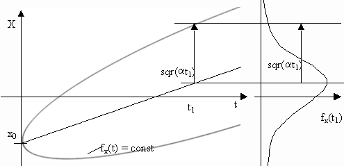
The probability density function for y(t) is the gaussian distribution with a mean value (y0+b t) and a time dependent variation a t.

The figure below demonstrates the evolution of the distribution function over time.
